To understand how trace elements partition between phases in the Earth, we use high pressure and temperature experiments to equilibrate the phases we’re interested in, then measure the element concentrations in each phase. We call the ratio of element concentrations in each phase the partition coefficient. By performing experiments at many different conditions (e.g., pressures, temperatures, phase compositions, redox), we can build a picture of how different variables control an elements partition coefficient. Often, we have to build this picture at conditions that are easy to achieve in the lab, then extrapolate our results to more extreme conditions. To do this, we parameterize the results of our experiments. Parameterization can be a useful tool, but it requires making some assumptions. If these assumptions are flawed, the extrapolated results won’t be accurate.
To parameterize metal-silicate partition coefficients we typically assume that cationic trace elements dissolve in the silicate melt as oxide species. Often, this is a safe assumption, as oxygen is usually the dominant anion in silicate melts (lavas/magmas). However, when the metal and silicate contain large amounts of sulfur some elements dissolve in the silicate melt as sulfide species. This can cause some added complications when parameterizing and then extrapolating experimental results.

Because the partitioning of both sulfur and many trace elements depends upon pressure, elements that form sulfide and oxide species in the silicate melt experience a coupled effect on their partition coefficient when pressure changes. The first effect arises from the volume change of reaction and the second from the availability of sulfur in the silicate melt to form sulfide species (there will also be effects arising from changes in the silicate and metallic melt composition, but for simplicity we will ignore those for now).
Figure 1 shows how the partition coefficient changes with pressure for a hypothetical element (i) that forms oxide and sulfide species in the silicate melt. The volume change of the elements reaction between metal and silicate is such that it should partition less strongly into the metal phase as pressure increases. This is exactly what is seen when there is no sulfur in the system (blue line). When there is sulfur in the system, however, the partition coefficient for element i initially increases as pressure increases. This happens because sulfur partitions more strongly into the metal as pressure increases. So, when we increase pressure, sulfur leaves the silicate melt and our trace element can no longer form sulfide species. Once the silicate melt is essentially sulfur free (~20 GPa in this example), element i behaves in the same way as in the sulfur-free system.
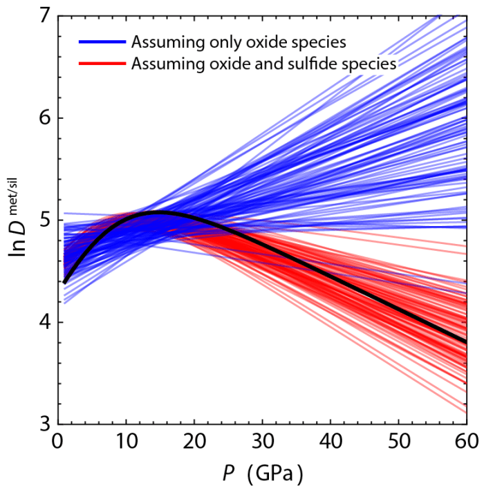
When experimental data are parameterized assuming only oxide species, a linear dependence of the partition coefficient on pressure is typically used. If the element forms oxide and sulfide species in the silicate melt, however, this can cause problems like those shown in Figure 2. The black line in Figure 2 shows how the partition coefficient changes with pressure for an element that forms sulfide and oxide species in the silicate melt. Using this behavior, I generated model datasets and then fit them with parameterizations that assume 1 species in silicate melt (blue lines) and 2 species in silicate melt (red lines). When only a single species is considered, the parameterization is acceptable at low pressures, but is not accurate when extrapolated to high pressures. Using the 2 species method I derived, that incorporates the effects of oxide and sulfide species, problems with extrapolating to high pressure are avoided.
So far, we have just looked at schematic behavior, in order to explore what problems may arise. Now, we can take what we’ve learnt and apply it to some real data. Figure 3 displays metal-silicate partitioning data for gold. Panel a displays data from sulfur-bearing experiments at a range of pressures and temperatures from a study by Righter et al., (2015). These data have been recalculated to a common metal composition, so that we can compare the experiments more directly. Just like with our model data in Figs 1 and 2, we see that the partition coefficient increases with pressure first, then decreases. In panel b, I have added the results of some sulfur-bearing low pressure experiments I performed, and also recalculated all the partition coefficients to a common temperature. The same increase, then decrease, in the partition coefficient with increasing pressure is observed. The black line in panel b is the best fit to these data using a 2-species relationship. The grey lines are similarly good fits at the 95% confidence level.
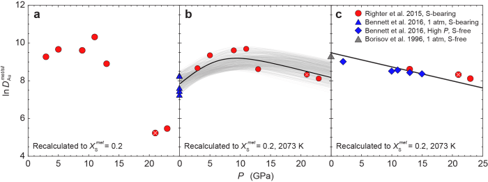
In panel c, we test the expectation that at high pressure, the sulfur-bearing experiments and sulfur-free experiments will be essentially the same and lie on a single linear trend. We see that this is in fact the case, which supports the idea that Au is forming oxide and sulfide species in the silicate melt. We still don’t know how important this type of behavior is for many elements, but it is most likely to play a role for other strongly chalcophile (sulfur-loving) elements, such as the platinum group metals and copper.
Associated Papers
Bennett, N. R. & Fei., Y. 2018. Pressure, sulfur, and metal-silicate partitioning: The effect of sulfur species on the parameterization of experimental results, American Mineralogist, 103, 1068-1079.
Bennett, N. R., Brenan, J. M., Fei, Y. 2016. Magma ocean thermometry: Controls on the metal-silicate partitioning of gold, Geochimica et Cosmochimica Acta, 184, 173-192.
